Why can't I just use impedance control on any geared motor?

Impedance control relies on backdrivability to regulate torque accurately. Highly geared motors (like harmonic drives > 100:1) have substantial friction and inertia, severely degrading torque transparency unless paired with a highly accurate torque sensor and very high-bandwidth control loops.

Is admittance control inherently slower than impedance control?

Often, yes. Because admittance control reads a force sensor, filters it, computes a virtual position, and feeds it into an inner position loop, it accumulates latency (phase lag). In hard contact situations, this latency can cause instability (bouncing).

Which control method requires an external 6-axis force-torque sensor?

Admittance control almost always requires an external force/torque sensor at the end-effector or joint to measure the environmental contact force, which serves as the input to the admittance model.

Can proprioception (current sensing) be used for admittance control?

Typically no. Admittance control is used on non-backdrivable systems where proprioceptive torque estimation (motor current) is highly inaccurate due to transmission friction. You need physical force sensors.

What is a 'hybrid' control approach?

A hybrid approach might use impedance control for backdrivable joints (like arms) to handle impacts gracefully, while using admittance control on highly geared joints (like wrists) for precise force-guided insertion tasks.

Admittance vs Impedance Control: Actuator & Hardware Differences

Executive Summary (Updated: 2026-09-24)

The choice between admittance vs impedance control is defined by hardware causality. Impedance control (Motion In → Force Out) dominates highly backdrivable, low-ratio systems. Admittance control (Force In → Motion Out) is required for stiff, high-ratio, non-backdrivable joints using external sensors. Choosing the wrong control paradigm for your actuator BOM will result in contact instability or unsafe hardware operation.

Request Architecture Review

1. Key Conclusions

To resolve the hardware and control divide, engineers must align the robotic task environment with the transmission physics.

1. Causality Inversion

Impedance treats the robot as a spring (input: displacement, output: force). Admittance treats it as a mass (input: force, output: displacement). They are mathematically inverse.

2. Hardware Dependency

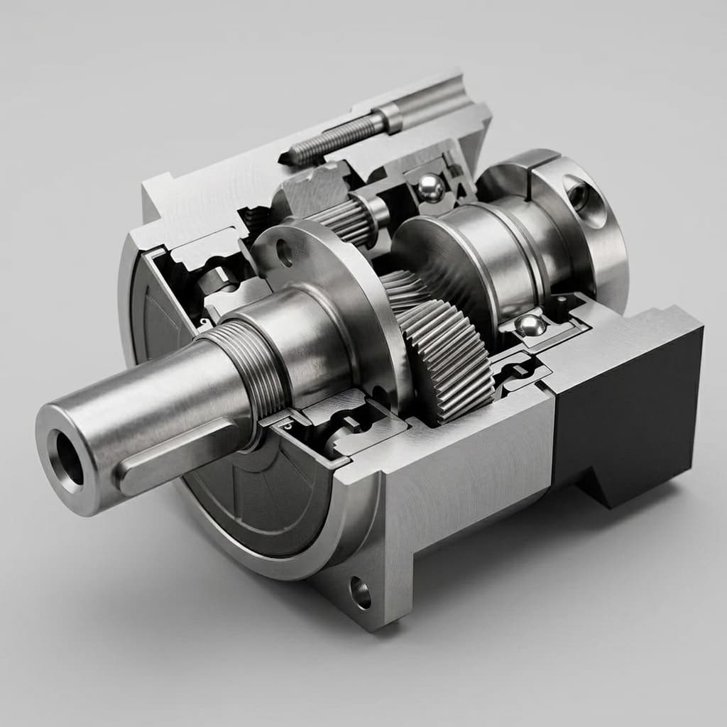
Impedance requires high backdrivability (low gear ratios, quasi-direct drive). Admittance is designed to force compliance onto stiff, non-backdrivable actuators (high-ratio harmonic drives).

3. Sensor Strategy

Admittance control heavily relies on external multi-axis force/torque (F/T) sensors. Impedance can often rely on motor current (proprioception) if the transmission is sufficiently transparent.

4. Contact Stability Limit

Admittance controllers struggle with hard environment contacts due to sensor-computation-actuation latency, often resulting in limit cycles (bouncing).

2. Structural Comparison: Impedance vs Admittance

A formal comparison based on mechanical causality and control loop implementation.

Dimension	Impedance Control	Admittance Control
Control Input (Measured)	Position / Velocity (Displacement)	Force / Torque (Contact)
Control Output (Command)	Force / Torque	Position / Velocity
Ideal Actuator Hardware	Direct-drive, Quasi-direct drive (low ratio < 10:1), SEA	High gear ratio (Harmonic, Cycloidal > 50:1)
Inner Loop Strategy	Fast current/torque loop (transparent)	Stiff position/velocity loop
Environmental Match	Environment acts as an Admittance (yielding/free space)	Environment acts as an Impedance (stiff constraints)

References: Baseline causality principles from fundamental robotics literature (e.g., Hogan 1985, Siciliano & Khatib).

System Causality Flow

3. Scope of Applicability & Boundaries

Not every robot can implement both control schemes effectively.

When to Use Impedance Control

Applicable Domains: Legged locomotion (quadrupeds, humanoid legs), dynamic manipulation, unconstrained path following with expected minor bumps.
Assumptions: The robot's actuators are highly transparent (low mechanical impedance). The environment is mostly unconstrained mass (free space).
Inapplicable Scenarios: High-precision, high-force rigid machining (e.g., robotic milling). Direct-drive motors lack the raw holding torque and stiffness needed for heavy industrial grinding.

When to Use Admittance Control

Applicable Domains: Industrial assembly (peg-in-hole), polishing/grinding, medical robotics where high-ratio actuators are mandatory for safety and payload.
Assumptions: The robot is mechanically stiff. The environment applies constraint forces that must be complied with. A high-quality external F/T sensor is installed.
Inapplicable Scenarios: High-speed impacts or running locomotion. The sensor-to-motor latency will cause the stiff limb to absorb the impact destructively before the software can "yield".

4. Risks, Limitations, and Trade-offs

Risk 1: Admittance Contact Instability

Trigger Condition: An admittance-controlled arm makes sudden contact with a very stiff environment (e.g., steel table).
Consequence: The time delay between force sensing and position yielding causes the controller to overcompensate, leading to violent oscillation.
Mitigation: Lower the virtual mass (though this is limited by actual system bandwidth), increase physical damping (soft fingertips), or increase loop execution rates (> 1kHz).

Risk 2: Impedance Torque Resolution Loss

Trigger Condition: Attempting pure impedance control on a 100:1 harmonic drive joint without a joint torque sensor.
Consequence: Static friction (stiction) dominates the drive. The current-to-torque mapping becomes non-linear, rendering the impedance model highly inaccurate in low-force scenarios.
Mitigation: Add explicit joint torque sensors or switch to an admittance paradigm using end-effector F/T sensors.

5. Actionable Advice for Next Steps

Whether you are a researcher, systems engineer, or hardware purchaser, your next steps vary based on your control choice:

For Systems Engineers: Audit your real-time network capability. If you are targeting impedance control, confirm that your EtherCAT (or similar) network supports cycle times $\le 1$ ms with minimal jitter.
For Hardware Procurement: If the software team mandates admittance control, budget for high-resolution 6-axis F/T sensors and stiff, high-ratio joints. If impedance is mandated, prioritize Quasi-Direct Drive (QDD) actuators or Series Elastic Actuators (SEA).
For Firmware Developers: Validate the current-loop bandwidth of your motor drivers. Impedance control requires high-bandwidth inner torque loops (> 1kHz) to simulate the desired mechanical compliance accurately.

Admittance vs Impedance Control: Architecture Decision Guide